Getting Started
In this section the basics of using the SWIFT-Emulator will be explained, with examples of how to make your first GP predictions.
Installation
The package can be installed easily from PyPI under the name swiftemulator, so:
pip3 install swiftemulator
This will install all necessary dependencies.
The package can be installed from source, by cloning the repository and then using pip install -e . for development purposes.
Requirements
The package requires a number of numerical and experimental design packages. These have been tested (and are continuously tested) using GitHub actions CI to use the latest versions available on PyPI. See requirements.txt for details for the packages required to develop SWIFT-Emulator. The packages will be installed automatically by pip when installing from PyPI.
Loading data
In the way we set up the emulator, loading the data is the most cumbersome part of emulation. Once everything is in the right format the emulation itself will be very easy.
At the basis of the SWIFT-Emulator lies the ability to train a Gaussian process (GP) based on a set of training data. As the main goal is emulating scaling relations on the back of hydro simulations you should think of the emulation being in the following form
where we want to predict the dependent \(y\) as a function of the independent \(x\) and model parameters \(\theta\). The distinction between \(x\) and \(\theta\) is made to distinquish the relation that can be obtained from a single simulation output (Like the number density of galaxies as a function of their stellar mass, where y is the number density and x the stellar mass) from the parameters that span different outputs (Like redshift, or AGN feedback strength). For this example we will predict the stellar mass function using some data generated with a Schecter function
import swiftemulator as se
import numpy as np

def log_schecter_function(log_M, log_M_star, alpha):
    M = 10 ** log_M
    M_star = 10 ** log_M_star
    return np.log10( (1 / M_star) * (M / M_star) ** alpha * np.exp(- M / M_star ))
where we set the normalisation to unity. In this case we will use log_M as the independent, while M_star and alpha are our model parameters. The choice to emulate in log space is important, this massively decreases the dynamic range which makes it a lot easier for a Gaussian process to emulate accurately.
In order to get the data in the correct form we need to
define three containers. We start by specifying some of the
basic information of our model. This is done via swiftemulator.backend.model_specification().
model_specification = se.ModelSpecification(
    number_of_parameters=2,
    parameter_names=["log_M_star","alpha"],
    parameter_limits=[[11.,12.],[-1.,-3.]],
    parameter_printable_names=["Mass at knee","Low mass slope"],
)
The mode specification is used to store some of the metadata of the training set.
Lets assume our training set consists of 100 simulations where our model parameters are randomly sampled
log_M_star = np.random.uniform(11., 12., 100)
alpha      = np.random.uniform(-1., -3., 100)
This can be used to set up the second container, which contains the model parameters. For each unique model, named by unique_identifier, we store the values in a dictionary
modelparameters = {}
for unique_identifier in range(100):
    modelparameters[unique_identifier] = {"log_M_star": log_M_star[unique_identifier],
                                        "alpha": alpha[unique_identifier]}

model_parameters = se.ModelParameters(model_parameters=modelparameters)
The unique_identifier is really important, as this will be used to link the model parameters to the model values. There are some major advantages to splitting this up. By splitting the model from the scaling relation we only have to define the model once, allowing us to attach as many relations to it as we want.
Final thing is adding the values of the function we want to emulate. This is done in a similar way to how we add the model parameters, except that we now attach a complete array for each model.
modelvalues = {}
for unique_identifier in range(100):
    independent = np.linspace(10,12,10)
    dependent = log_schecter_function(independent,
                                      log_M_star[unique_identifier],
                                      alpha[unique_identifier])
    dependent_error = 0.02 * dependent
    modelvalues[unique_identifier] = {"independent": independent,
                                    "dependent": dependent,
                                    "dependent_error": dependent_error}

model_values = se.ModelValues(model_values=modelvalues)
For the model values it is important that you use the names independent, dependent and dependent_error for x, y and y_err respectively. These specific names are used when setting up the emulator
Training the emulator
After setting up de model containers, training the emulator becomes very simple. First we create an empty GP, which we can then train on the data we have just loaded.
from swiftemulator.emulators import gaussian_process
schecter_emulator = gaussian_process.GaussianProcessEmulator()
schecter_emulator.fit_model(model_specification=model_specification,
                            model_parameters=model_parameters,
                            model_values=model_values)
This might take a little bit of time. At this point the GP is fully trained and can be used to make predictions. There are a lot more options when setting up the GP, like indlucing a model for mean, but if your input is smooth this is likely all you will need.
Making predictions
The real reason to use an emulator is to eventually predict the shape of the scaling relation continuously over the parameterspace. Just like training the emulator, making predictions is extremely simple
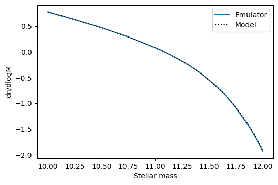
predictparams = {"log_M_star": 11.5, "alpha": -2}
predict_x = np.linspace(10,12,100)

pred, pred_var = schecter_emulator.predict_values(predict_x, predictparams)
The main thing to keep in mind is that you give the model parameters as a dictionary again, with the same names as how they are defined in the model_parameters. In this case we can directly compare with the original model.
import matplotlib.pyplot as plt
plt.plot(predict_x,pred,label="Emulator")
plt.plot(predict_x,log_schecter_function(predict_x,
                                        predictparams["log_M_star"]
                                        ,predictparams["alpha"])
        ,color="black",ls=":",label="Model")
plt.xlabel("Stellar mass")
plt.ylabel("dn/dlogM")
plt.legend()
Which shows that the emulator can predict the model with high accuracy.
This covers the most basic way to use SWIFT-Emulator and should give a good baseline for using some of the additional features it offers.