Comparing With Data
To unlock the full power of emulation it
is often usefull to compare your results
with observational data. With
SWIFT-Emulator you can directly compare
the emulated outputs with the observational
data stored in velociraptor-comparison-data
which can be found
here.
You can also download just the required Vernon.hdf5 file
instead.
In this case we will again use the data from http://virgodb.cosma.dur.ac.uk/swift-webstorage/IOExamples/emulator_output.zip First we have to set up the emulator
from swiftemulator.io.swift import load_parameter_files, load_pipeline_outputs
from swiftemulator.emulators.gaussian_process import GaussianProcessEmulator
from swiftemulator.mean_models import LinearMeanModel
from velociraptor.observations import load_observations

from glob import glob
from pathlib import Path
from tqdm import tqdm
from matplotlib.colors import Normalize

import matplotlib.pyplot as plt
import numpy as np
import corner

import os

files = [Path(x) for x in glob("./emulator_output/input_data/*.yml")]

filenames = {filename.stem: filename for filename in files}

spec, parameters = load_parameter_files(
    filenames=filenames,
    parameters=[
        "EAGLEFeedback:SNII_energy_fraction_min",
        "EAGLEFeedback:SNII_energy_fraction_max",
        "EAGLEFeedback:SNII_energy_fraction_n_Z",
        "EAGLEFeedback:SNII_energy_fraction_n_0_H_p_cm3",
        "EAGLEFeedback:SNII_energy_fraction_n_n",
        "EAGLEAGN:coupling_efficiency",
        "EAGLEAGN:viscous_alpha",
        "EAGLEAGN:AGN_delta_T_K",
    ],
    log_parameters=[
        "EAGLEAGN:AGN_delta_T_K",
        "EAGLEAGN:viscous_alpha",
        "EAGLEAGN:coupling_efficiency",
        "EAGLEFeedback:SNII_energy_fraction_n_0_H_p_cm3",
    ],
    parameter_printable_names=[
        "$f_{\\rm E, min}$",
        "$f_{\\rm E, max}$",
        "$n_{Z}$",
        "$\\log_{10}$ $n_{\\rm H, 0}$",
        "$n_{n}$",
        "$\\log_{10}$ $C_{\\rm eff}$",
        "$\\log_{10}$ $\\alpha_{\\rm V}$",
        "AGN $\\log_{10}$ $\\Delta T$",
    ],
)

value_files = [Path(x) for x in glob("./emulator_output/output_data/*.yml")]

filenames = {filename.stem: filename for filename in value_files}

values, units = load_pipeline_outputs(
    filenames=filenames,
    scaling_relations=["stellar_mass_function_100"],
    log_independent=["stellar_mass_function_100"],
    log_dependent=["stellar_mass_function_100"],
)

# Train an emulator for the space.
scaling_relation = values["stellar_mass_function_100"]
scaling_relation_units = units["stellar_mass_function_100"]

emulator = GaussianProcessEmulator()
emulator.fit_model(model_specification=spec,
    model_parameters=parameters,
    model_values=scaling_relation,
)
In this case we are gonna look at the stellar mass function. To compare we load the calibration SMF for EAGLE-XL.
observation = load_observations(
    "../velociraptor-comparison-data/data/GalaxyStellarMassFunction/Vernon.hdf5"
)[0]
Penalty Functions
There is a large selection of “Penalty” functions available. We define a penalty function as an analogous to a likelihood.
where \(\mathcal{L}\) is the likelihood and \(P(x,\theta)\) is the accompanying penalty function.
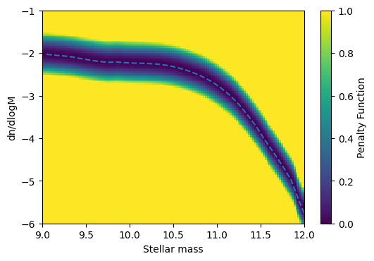
As an example we will use an L2 norm. This will calculate the mean squared distance between the emulator and the data.
from swiftemulator.comparison.penalty import L2PenaltyCalculator
from unyt import Msun, Mpc

L2_penalty = L2PenaltyCalculator(offset = 0.5, lower=9,upper=12)
L2_penalty.register_observation(observation,log_independent=True
                            ,log_dependent=True
                            ,independent_units=Msun
                            ,dependent_units=Mpc**-3)

L2_penalty.plot_penalty(9,12,-6,-1,"penalty_example",x_label="Stellar mass",y_label="dn/dlogM")
Now we can combine this with the emulator to compare models
in terms of how good they fit the data. Without using the
emulator we can use interpolation to be able to quickly check
which node of the parameter space best fits the data via
swiftemulator.comparison.penalty.L2PenaltyCalculator.penalties()
all_penalties = L2_penalty.penalties(emulator.model_values,np.mean)

all_penalties_array = []
node_number = []
for key in all_penalties.keys():
    all_penalties_array.append(all_penalties[key])
    node_number.append(int(key))

print("Best fit node = ",node_number[np.argmin(all_penalties_array)])
Best fit node = 107
If we want to check the simulation that is best without rerunning anything we can use node 107. In general we can use this to check not just models at the nodes, but use the emulator to check the complete parameter range. Starting with node 107, let’s see if we can improve the fit by chaning one of the parameters.
predictparams = emulator.model_parameters["107"].copy()
x_to_predict = np.log10(L2_penalty.observation.x.value)
pred, pred_var = emulator.predict_values(x_to_predict, predictparams)

print("Mean Penalty of node 107 = ",np.mean(L2_penalty.penalty(x_to_predict,pred)))

#Let's change one of the parameters and see if it improves the fit
predictparams["EAGLEFeedback:SNII_energy_fraction_max"] = 1
x_to_predict = np.log10(L2_penalty.observation.x.value)
pred, pred_var = emulator.predict_values(x_to_predict, predictparams)

print("Mean after change = ",np.mean(L2_penalty.penalty(x_to_predict,pred)))
Mean Penalty of node 107 =  0.21988119507121354
Mean after change =  0.3344361855742612
This change makes the fit worse, so no luck. In general you would not do this by hand, but use for example MCMC to sample all the parameters.
Defining New Penalty Functions
What you want out of these penalty functions can vary wildy,
but it is very easy to define your own. There is a large set
of functions available within
swiftemulator.comparison.penalty(). It is also possible
to add your own functions. The base class
swiftemulator.comparison.penalty.PenaltyCalculator()
covers the most important part, which is loading and
interpolating the data. You can then add whichever calculattion
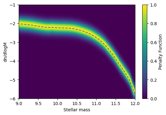
of the penalties you want. In the example below we create a
function that is Gaussian weighted, with a constent error
term.
from swiftemulator.comparison.penalty import PenaltyCalculator
import unyt

class ExamplePenaltyCalculator(PenaltyCalculator):

    def penalty(self,independent, dependent, dependent_error):
        #We can use the observational data from the base class.
        #We calculate the observational y-values to compare with
        #from the interpolated observations.
        obs_dependent = self.interpolator_values(independent)

        penalties = np.exp(-np.abs(dependent - obs_dependent)**2/0.1)
        return penalties

my_penalty = ExamplePenaltyCalculator()
my_penalty.register_observation(observation,log_independent=True,log_dependent=True
                            ,independent_units=Msun,dependent_units=Mpc**-3)

my_penalty.plot_penalty(9,12,-6,-1,"my_penalty",x_label="Stellar mass",y_label="dn/dlogM")
For the simplest models you can also still use the plot_penalty
functionality. There are also PF’s available that use the
errors on the data, for example
swiftemulator.comparison.penalty.GaussianDataErrorsPenaltyCalculator().
When creating new penalty functions you can use different parts
of already existing ones to make the process very easy.